Manuscript/Report Template for a Data Analysis Project

The structure below is one possible setup for a data analysis project (including the course project). For a manuscript, adjust as needed. You don’t need to have exactly these sections, but the content covering those sections should be addressed.

This uses MS Word as output format. See here for more information. You can switch to other formats, like html or pdf. See the Quarto documentation for other formats.

Warning: package 'knitr' was built under R version 4.4.2

1 Summary/Abstract

Write a summary of your project.

2 Introduction

2.1 General Background Information

Provide enough background on your topic that others can understand the why and how of your analysis

2.2 Description of data and data source

The data contains a combination of numeric and categorical data related to people. There are four columns, these look into height, gender, minutes of daily exercise, and star/zodiac sign.

2.3 Questions/Hypotheses to be addressed

State the research questions you plan to answer with this analysis.

To cite other work (important everywhere, but likely happens first in introduction), make sure your references are in the bibtex file specified in the YAML header above (here dataanalysis_template_references.bib) and have the right bibtex key. Then you can include like this:

Examples of reproducible research projects can for instance be found in (McKay, Ebell, Billings, et al., 2020; McKay, Ebell, Dale, Shen, & Handel, 2020)

3 Methods

Describe your methods. That should describe the data, the cleaning processes, and the analysis approaches. You might want to provide a shorter description here and all the details in the supplement.

3.1 Data aquisition

As applicable, explain where and how you got the data. If you directly import the data from an online source, you can combine this section with the next.

3.2 Data import and cleaning

Write code that reads in the file and cleans it so it’s ready for analysis. Since this will be fairly long code for most datasets, it might be a good idea to have it in one or several R scripts. If that is the case, explain here briefly what kind of cleaning/processing you do, and provide more details and well documented code somewhere (e.g. as supplement in a paper). All materials, including files that contain code, should be commented well so everyone can follow along.

3.3 Statistical analysis

Explain anything related to your statistical analyses.

4 Results

4.1 Exploratory/Descriptive analysis

Use a combination of text/tables/figures to explore and describe your data. Show the most important descriptive results here. Additional ones should go in the supplement. Even more can be in the R and Quarto files that are part of your project.

Table 1 shows a summary of the data.

Note the loading of the data providing a relative path using the ../../ notation. (Two dots means a folder up). You never want to specify an absolute path like C:\ahandel\myproject\results\ because if you share this with someone, it won’t work for them since they don’t have that path. You can also use the here R package to create paths. See examples of that below. I recommend the here package, but I’m showing the other approach here just in case you encounter it.

Table 1: Data summary table.

skim_type	skim_variable	n_missing	complete_rate	character.min	character.max	character.empty	character.n_unique	character.whitespace	factor.ordered	factor.n_unique	factor.top_counts	numeric.mean	numeric.sd	numeric.p0	numeric.p25	numeric.p50	numeric.p75	numeric.p100	numeric.hist
character	Star sign	0	1	5	9	0	7	0	NA	NA	NA	NA	NA	NA	NA	NA	NA	NA	NA
factor	Gender	0	1	NA	NA	NA	NA	NA	FALSE	3	M: 4, F: 3, O: 2	NA	NA	NA	NA	NA	NA	NA	NA
numeric	Height	0	1	NA	NA	NA	NA	NA	NA	NA	NA	165.66667	15.97655	133	156	166	178	183	▂▁▃▃▇
numeric	Weight	0	1	NA	NA	NA	NA	NA	NA	NA	NA	70.11111	21.24526	45	55	70	80	110	▇▂▃▂▂
numeric	Daily Exercise minutes	0	1	NA	NA	NA	NA	NA	NA	NA	NA	18.77778	18.06085	0	7	15	22	60	▇▆▂▁▂

4.2 Basic statistical analysis

To get some further insight into your data, if reasonable you could compute simple statistics (e.g. simple models with 1 predictor) to look for associations between your outcome(s) and each individual predictor variable. Though note that unless you pre-specified the outcome and main exposure, any “p<0.05 means statistical significance” interpretation is not valid.

Figure 1 shows a scatterplot figure produced by one of the R scripts.

Figure 1: Height and weight stratified by gender.

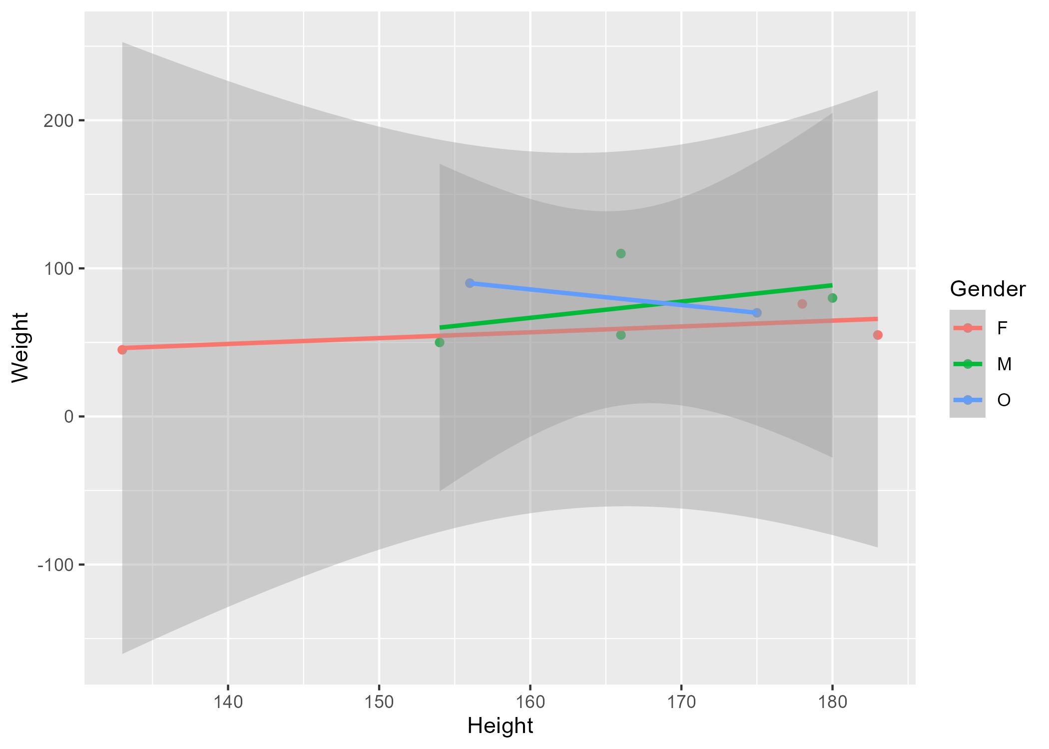
Figure 2 shows a scatterplot figure evaluating weight and daily exercise minutes as produced by one of the R scripts.

Figure 2: Weight and daily exercise minutes.

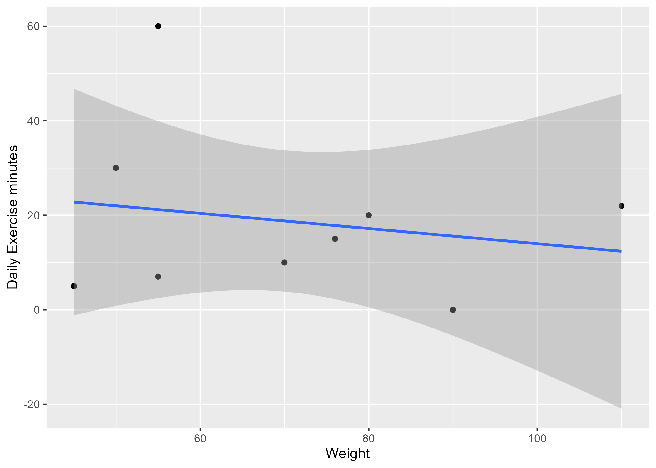
The figure seems to demonstrate a negative correlation between daily exercise and weight, as daily exercise minutes increase, weight decreases.

Figure 3 shows a boxplot figure evaluating star sign and height as produced by one of the R scripts.

Figure 3: Star sign and height.

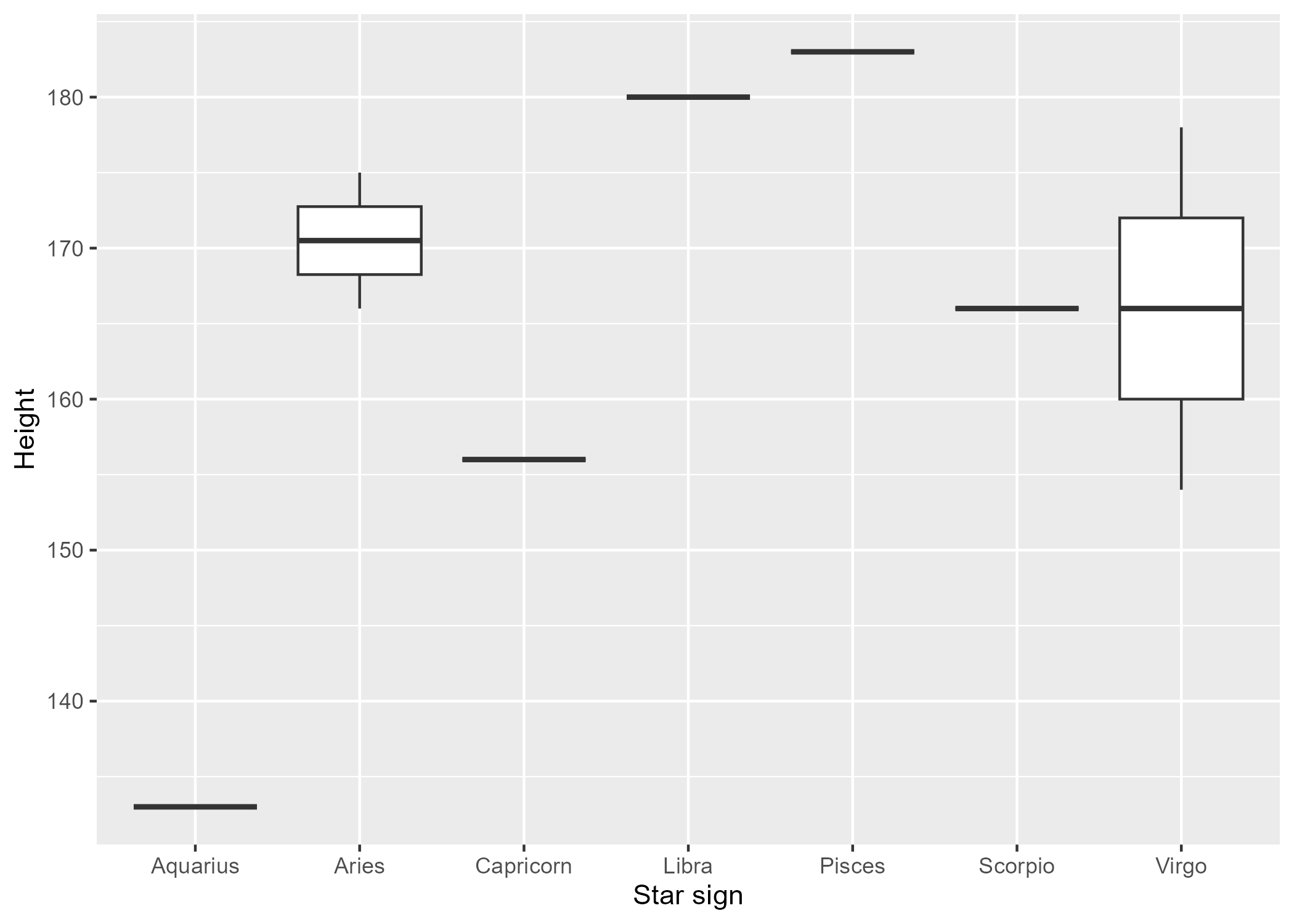
The box plot does not indicate much information regarding a relationship between star (zodiac) sign and height, and this is likely because there are too few data points to evaluate this effectively. We do see that most participants (except for one) were over 155cm in height and that Virgo was the most common star sign in the dataset.

4.3 Full analysis

Use one or several suitable statistical/machine learning methods to analyze your data and to produce meaningful figures, tables, etc. This might again be code that is best placed in one or several separate R scripts that need to be well documented. You want the code to produce figures and data ready for display as tables, and save those. Then you load them here.

Example Table 2 shows a summary of a linear model fit.

Table 2: Linear model fit table.

term	estimate	std.error	statistic	p.value
(Intercept)	149.2726967	23.3823360	6.3839942	0.0013962
Weight	0.2623972	0.3512436	0.7470519	0.4886517
GenderM	-2.1244913	15.5488953	-0.1366329	0.8966520
GenderO	-4.7644739	19.0114155	-0.2506112	0.8120871

Example Table 3 shows a summary of a linear model fit for height as an outcome with daily exercise minutes and star sign as predictors.

Table 3: Linear model fit table.

term	estimate	std.error	statistic	p.value
(Intercept)	139.341463	6.0014622	23.217919	0.0274024
Daily Exercise minutes	-1.268293	0.4146341	-3.058823	0.2011529
Star signAries	51.451220	8.2693269	6.221936	0.1014510
Star signCapricorn	16.658537	8.2302528	2.024061	0.2921329
Star signLibra	66.024390	10.1055112	6.533503	0.0966889
Star signPisces	52.536585	8.0079155	6.560582	0.0962959
Star signScorpio	102.756098	24.1557754	4.253894	0.1469870
Star signVirgo	55.195122	10.0115044	5.513170	0.1142306

There does not seem to be a statistically significant association between these factors.

5 Discussion

5.1 Summary and Interpretation

Summarize what you did, what you found and what it means.

5.2 Strengths and Limitations

Discuss what you perceive as strengths and limitations of your analysis.

5.3 Conclusions

What are the main take-home messages?

Include citations in your Rmd file using bibtex, the list of references will automatically be placed at the end

This paper (Leek & Peng, 2015) discusses types of analyses.

These papers (McKay, Ebell, Billings, et al., 2020; McKay, Ebell, Dale, et al., 2020) are good examples of papers published using a fully reproducible setup similar to the one shown in this template.

Note that this cited reference will show up at the end of the document, the reference formatting is determined by the CSL file specified in the YAML header. Many more style files for almost any journal are available. You also specify the location of your bibtex reference file in the YAML. You can call your reference file anything you like, I just used the generic word references.bib but giving it a more descriptive name is probably better.

6 References

Leek, J. T., & Peng, R. D. (2015). Statistics. What is the question? Science (New York, N.Y.), 347(6228), 1314–1315. https://doi.org/10.1126/science.aaa6146

McKay, B., Ebell, M., Billings, W. Z., Dale, A. P., Shen, Y., & Handel, A. (2020). Associations Between Relative Viral Load at Diagnosis and Influenza A Symptoms and Recovery. Open Forum Infectious Diseases, 7(11), ofaa494. https://doi.org/10.1093/ofid/ofaa494

McKay, B., Ebell, M., Dale, A. P., Shen, Y., & Handel, A. (2020). Virulence-mediated infectiousness and activity trade-offs and their impact on transmission potential of influenza patients. Proceedings. Biological Sciences, 287(1927), 20200496. https://doi.org/10.1098/rspb.2020.0496